
All sciences. №3, 2023. International Scientific Journal

Table 1. A series of long numbers for interesting values of numbers-granules (the first line is the original value)
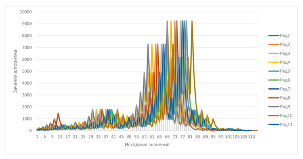
Fig. 1. Graph of values for interesting numbers-granules of the algorithm
When the path of one number is so much different even from the neighboring one, how do you even approach the proof of such a hypothesis? Of course, all mathematicians were at a loss and absolutely no one could solve this problem. So Jeffrey Lagarias is a world expert on this problem, and he said that no one should take up this problem if he wants to become a mathematician. A large-scale work was carried out and a huge number of hailstones were studied, trying to find a pattern. Here it can be argued that all values come to one, however, what can be said about the path that all numbers take? The interesting thing is that this path is absolutely random.
For example, we can give a graph of all the values of this algorithm from 1 to 100 (Fig. 2).
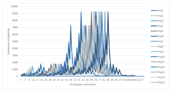
Fig. 2. Graph of values for numbers-granules from 1 to 100
As you can see, most often growth begins initially and after a sharp decline, while the value of the number is simply not considered, however, if you make the graph logarithmic, there is a downward trend in its fluctuations. It can also be observed on the stock market on the day of the collapse, which is not accidental, because these are examples of geometric Brownian motion, that is, if you take logarithms and calculate the linear component, the fluctuations seem random, as if a coin was thrown at each step. And if we consider this function analysis as part of mathematical analysis, then there begins to be an obvious connection with probability theory. From where it turns out that when heads are obtained, the line goes up, and when tails go down, from where a special graph is obtained.
If we consider this chart when compared with the same exchange, then it is more likely in a short-term analysis, although in the long term, stocks are still growing, and "3x+1" is falling. You can also pay attention to the highest digit of the gradient numbers – this means a histogram, which is obtained by counting the number of digits from which the numbers begin in a number of granules for a particular number of the algorithm. If you add these values each time, for 1, 2, 3, etc., more and more data is obtained, while the ratio of the height of the columns becomes more and more ordered.
So for the first billion sequences, the most frequent value is one, 29.94% of all cases, 2 – 17,47%, 3 – 12,09%, 4 – 10,63%, 5 – 7,94%, 6 – 6,16%, 7 – 5,76%, 8 – 5,31%, 9 – 4,7% and the larger the figure, the less often it turns out to be ahead.
This arrangement is typical not only for hailstone numbers, there are many examples, these are the population of countries, the value of companies, all physical constants or Fibonacci numbers, and much more. This law is called Benford's law. Surprisingly, if you trace the violation of the Benford law in tax returns, you can even determine the fact of fraud. This law also helps to identify anomalies in the counting of votes in elections or many other things.
The best effect of this law occurs when the numbers entered in it have a spread of several orders of magnitude, as in this case, but Benford's law, unfortunately, cannot tell whether all the numbers end up in the 4-2-1 cycle. To do this, you need to use a different method. Initially, it is strange that this algorithm reduces all numbers to 1, given that even and non-even numbers equally and non-even numbers increase by more than 3 times, and even numbers decrease by 2 times.
This suggests the conclusion that all sequences should, in theory, go up, not down. But it is worth paying attention to the fact that whenever an operation is performed with a non-even number, that is, when it is multiplied by 3 and 1 is added, it necessarily turns into an even number, therefore, the next step it will always be divided by 2. It turns out that non-even numbers are not tripled, but multiplied by (3x+1) /2 or more precisely by 1.5, because 0.5 for large numbers can be ignored. So the maximum growth from this is exactly 1.5.
A graph has already been given for all numbers from 1 to 100, but it is worth considering a small case for all non-even numbers. As you know, in the second step they turn into even values, and then exactly half of them are immediately reduced, after dividing again to non-even. But every 4 numbers will have to be divided by 2 twice, which means that these non-even numbers are ¾ of the previous one. Every 8th number will have to be divided by 2 three times to get an even number. Every 16 four times, etc.
So taking the geometric mean, you can see that in order to get from one non-even number to another through all even numbers, you need to multiply it by ¾, which is less than one, hence it turns out that statistically, this sequence decreases more often than it grows.
Let's give an example for a large number, for example 341. Its row looks like this:
341 – 1024 – 512 – 256 – 128 – 64 – 32 – 16 – 8 – 4 – 2 – 1.
He had only one non-even and all even numbers, which is why this series is remarkable. However, they can be depicted both in the form of graphs and in the form of trees, showing how one of the numbers is connected with the next in its sequence, creating a graph.
And if the hypothesis is correct, then any number should be in this huge graph, consisting of an infinite number of "streams" forming 4-2-1 cycles in one stream. There is an interesting visualization of such a graph, which uses an algorithm that on non—even numbers, it rotates clockwise at the selected angle, and counterclockwise on even numbers.
As a result, an interesting curved structure is obtained, more often in one direction. Resembling coral, algae or a tree in the wind. But this is only for a small number of numbers, for huge arrays, changing the angles of rotation, you can create huge and dazzlingly beautiful figures, as if generated by nature.
The hypothesis seems to be incorrect only in 2 cases:
1. If a number is found that will give infinity in the algorithm, that is, for some unknown reason, this "force of attraction" to 4-2-1 should not act on it;
2. Somewhere there is a sequence that would form its own closed loop, and all the numbers in it should be outside the main graph.
However, none of these options has been found yet, although all numbers up to 2 to the 68th power have already been checked by a simple search, which equals 295,147,905,179,352,825,856 numbers. It is known for sure that all the numbers from these values come to the 4-2-1 cycle. Moreover, based on these data, it is calculated that even if there is such a special data cycle, it should consist of at least 186 billion numbers. And it turns out that all the works indicate that the hypothesis is true, but still does not prove it.
Another way was also chosen. A scattering graph was constructed by taking the numbers themselves on one axis and the values on the other. If it can be proved that in any sequence of the algorithm there is a number smaller than the original one, it is possible to confirm the Collatz hypothesis. But any initial number is reduced to a smaller number, which in its own sequence will lead to a number even smaller, etc., up to 1.
That is, the only possible outcome for this particular case is the 4-2-1 cycle, but it has not yet been possible to prove this.
Although in 1976, Riho Terras showed that almost all sequences include values below the original one. In 1979, it was shown that the values would be less than the original ones by these values raised to the power of 0.869. Later, in 1994, the degree became more precise – 0.7925. Here, almost all the numbers mean that when the initial values tend to infinity, the proportion of the limiting function tends to 1. In 2019, mathematician Terry Tao was able to prove that this algorithm obeys even stricter restrictions.
He managed to show that all numbers will be less than the values of the function at any point, provided that the limit of the function, when the variable tends to infinity, will be equal to infinity. In this case, the function can grow arbitrarily slowly, the same logarithm, or logarithm logarithm, or logarithm logarithm, etc. This allows us to assert that arbitrarily small numbers exist in the series of any initial number. And as it was said in 2020, only a direct proof of the hypothesis can be better than this.
Used literature
1. Hayes, Brian. The ups and downs of hailstone numbers. American. – 1984. – No. 3. – pp. 102-107.
2. Stewart, Ian. The greatest mathematical problems. – M.: Alpina non-fiction, 2015. – 460 p.
3. Jeff Lagarias. The 3x+1 and its generalizations. American Mathematical Monthly. – 1985. – Vol. 92. – P. 3—23.
GENERAL IDEA OF THE CONCEPT AND USE OF DIFFERENTIAL EQUATIONS IN THE DESCRIPTION OF SOME DYNAMIC PHENOMENA
Aliev Ibratjon Khatamovich
2nd year student of the Faculty of Mathematics and Computer Science of Fergana State University
Ferghana State University, Ferghana, Uzbekistan
Аннотация. Как некогда сказал Стивен Строгац: «Со времён Ньютона человечество пришло к осознанию того, что физики выражаются на языке дифференциальных уравнений». Разумеется, что данный язык используется далеко за пределами физики и талант использовать его, ровно, как и воспринимать, даёт новые краски при изучении окружающего мира. В настоящей работе описывается общее представление об этом методе и сам процесс его изучения.
Ключевые слова: дифференциальные уравнения, исчисления, алгоритмы, математическая физика.
Annotation. As Stephen Strogatz once said: «Since the time of Newton, mankind has come to realize that physicists are expressed in the language of differential equations.» Of course, this language is used far beyond physics and the talent to use it, exactly as to perceive it, gives new colors when studying the surrounding world. This paper describes a general idea of this method and the process of studying it.
Keywords: differential equations, calculus, algorithms, mathematical physics.
By themselves, differential equations arise every time it is easier to describe a change than absolute values. For example, it is easier to describe the nature of an increase or decrease in the growth or decline of the population or population of a particular species than to describe certain values at a certain point in time. In physics, more precisely in Newtonian mechanics, motion is described by force, and force is determined by constant mass and changing acceleration, which is a statement of change.
Differential equations are divided into 2 large categories – ordinary differential equations or ODES involving functions with one variable, most often in the face of time and partial differential equations with several variables. If partial differential equations describe more complex characteristics, for example, temperature changes at different points in space, then ordinary differential equations describe more static characteristics that change over time.
As a good example, we can consider the process of falling of an object. As you know, the gravitational acceleration is 9.81 m/s2, which means that if you analyze the position of the body at every second and translate this state into vectors, they will accumulate an additional downward acceleration of 9.81 m/s2 every second. This gives an example of the simplest differential equation, the solution of which is the function y (t), the derivative of which gives the vertical component, and the velocity gives the vertical component of acceleration (1).

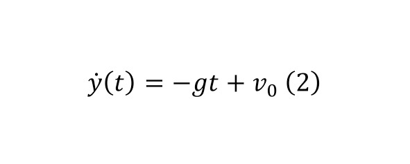
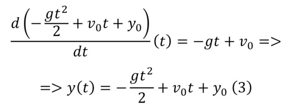
This equation can be solved by allocating (2) for speed and (3) for path.
Another interesting moment is when it is possible to describe the movement of celestial objects on this scale due to the force of gravity. So, two bodies are given whose attraction is directed towards each other with a force inversely proportional to the square of the distance between them (4).
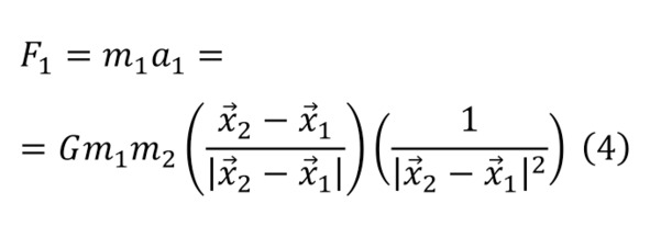
It is known that the derivative of the coordinate is velocity, the derivative of velocity is acceleration and it is necessary to obtain a function for motion, but according to equation (4), only the equation for acceleration (5) is known.

It may be strange here that the derivative is equal to the same function, but this is a common phenomenon when the derivative of the first or higher orders is determined by the values of themselves. But in practice, it is more often necessary to work with second-order differential equations, as can be seen in the previous examples.
However, there are also differential equations with third (6) or fourth (7) derivatives or higher (8) derivatives, which are considered higher-order differential equations.


In a way, it turns out that you need to find infinitely many numbers, one for each moment of time, but in general this coincides with the description of the function. And most often, even if in many cases it is possible to apply the classical description, then to a greater extent the use of the technology of ordinary mathematical transformations no longer meets the requirements. The usual description of the characteristics of a mathematical pendulum can be a proof of this.
Considering the real and idealized case, it can be noted that idealization works only at small angles of deflection of the pendulum, but when the angle becomes large enough, for example, equal to a semicircle, then the graph describing its oscillations as a whole ceases to be similar to the graphs of sine or cosine. The reason for this is the need to describe its motion exclusively using not partial, but general equations of harmonic oscillations with second-order differential equations.
This analogy can be applied to many other physical, most often real phenomena.
Used literature
1. Pontryagin L. S. Ordinary differential equations. – M.: Nauka, 1974.
2. Tikhonov A. N., Samarsky A. A. Equations of mathematical physics. – M.: Nauka, 1972.
3. Tikhonov A. N., Vasilyeva A. B., Sveshnikov A. G. Differential equations. – 4th ed. – Fzimatlit, 2005.
4. Umnov A. E., Umnov E. A. Fundamentals of the theory of differential equations. – Ed. 2nd – 2007. – 240 p.
5. Charles Henry Edwards, David E. Penny. Differential Equations and the problem of eigenvalues: Modeling and calculation using Mathematica, Maple and MATLAB = Differential Equations and Boundary Value Problems: Computing and Modeling. – 3rd ed. – M.: "Williams", 2007.
6. Elsholts L. E. Differential Equations and Calculus of Variations. – M.: Science, 1969.
ON THE ISSUES OF THE STUDY OF TRIPLE INTEGRALS
Aliev Ibratjon Khatamovich
2nd year student of the Faculty of Mathematics and Computer Science of Fergana State University
Ferghana State University, Ferghana, Uzbekistan
Аннотация. Изучение математической теории, способной в качестве отдельного инструмента описывать наблюдаемый мир весьма необходимо не только для исследователей в данной области, но и для всех представителей человеческой цивилизации, не говоря уже о тех, кто хочет производить описания математических теорий, ради этих же математических теорий. Особенной в данной части является такой метод исследования, как использование тройного или трёхкратного интеграла, наряду с отдельными операциями с элементами под знаком этого же тройного интеграла.
Ключевые слова: трёхкратные интегралы, математический анализ, исследования, определение, вычисление, научная новизна.
Annotation. The study of a mathematical theory capable of describing the observable world as a separate tool is very necessary not only for researchers in this field, but also for all representatives of human civilization, not to mention those who want to produce descriptions of mathematical theories for the sake of these same mathematical theories. Special in this part is such a method of research as the use of a triple or triple integral, along with separate operations with elements under the sign of the same triple integral.
Keywords: triple integrals, mathematical analysis, research, definition, calculation, scientific novelty.
The need to determine the volume, therefore, based on density and mass, along with the number of components and other derivatives of these quantities for objects that cannot be determined practically, a vivid example of this is the determination of the mass of a mountain, huge details for which it is not possible or too costly to use the Archimedes method, but it is necessary to calculate the volume or even when determining parameters of the whole planet.
The object of the study is a three-fold integral. The subject of the study is the process of calculating a triple integral, as well as operating with it when replacing variables of this triple integral. As a result of the study, some hypothesis is put forward that asserts the possibility of using triple integrals in calculating the parameters of linear accelerators relative to the internal particles of smooth electromagnetic waveguides of linear accelerators.
The objectives of the study are:
· Definition of the concept of a triple integral;
· Study of the process of replacing variables in a triple integral;
· Showing a model for calculating parameters by means of a three-fold integral for a linear accelerator waveguide.
The objectives of the study are:
· Study of the concept of a three-fold integral in the general understanding and some coordinate systems, indicating general concepts in a brief form;
Конец ознакомительного фрагмента.
Текст предоставлен ООО «ЛитРес».
Прочитайте эту книгу целиком, купив полную легальную версию на ЛитРес.
Безопасно оплатить книгу можно банковской картой Visa, MasterCard, Maestro, со счета мобильного телефона, с платежного терминала, в салоне МТС или Связной, через PayPal, WebMoney, Яндекс.Деньги, QIWI Кошелек, бонусными картами или другим удобным Вам способом.
Вы ознакомились с фрагментом книги.
Для бесплатного чтения открыта только часть текста.
Приобретайте полный текст книги у нашего партнера:
Всего 10 форматов